
Six million locations filtered in 14.7 ms by 8DB's preloaded kernel. The same campaign recorded 140 ms for DuckDB, 470 ms for SedonaDB and 13,140 ms for GeoPandas query paths.
These are recorded results with different measurement boundaries: 8DB times filtering and counting prepared coordinates; the reconstructed competitor paths include reading and returning query results. The comparison below shows the tested versions and scope.
For teams building location-aware applications, there are two stories worth exploring: how quickly the spatial core can run, and what becomes possible when location lives beside the rest of the application's data.
Five seconds, twenty-four seconds, or a ten-minute cutoff
SpatialBench Q12 asks for the five nearest buildings to each trip pickup. The May 7 SF1 campaign used six million trips and 20,000 buildings on a reported AWS m7i.2xlarge with eight vCPUs and 32 GB RAM.
| Recorded Q12 path | Reported elapsed time | Recorded outcome |
|---|---|---|
| 8DB R-tree kernel | 5.20 s | Counted 30 million candidate pairs |
| SedonaDB 0.3.0 query | 23.88 s | Reported 30 million result rows |
| DuckDB 1.5.2 query | 600-second cutoff | Timed out |
| GeoPandas 1.1.3 query | 600-second cutoff | Timed out |
Ten minutes without a completed answer matters when a workflow is waiting on the result. Here, the timeout applies to the tested DuckDB and GeoPandas configurations; SedonaDB completed the query.
Open the original nearest-neighbor timing chart.
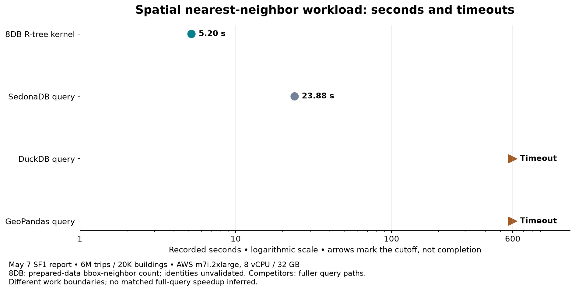
For 8DB, the 5.20-second result demonstrates a fast candidate-search path. Its timer excludes preparation, and the recovered implementation counts neighbors from a building bounding-box index rather than returning the full ordered polygon-distance result. Thirty million pairs is the expected count, but does not prove the same neighbor identities. These differences prevent translating the table into a matched full-query speedup. Original campaign report.
The engineering opportunity is to carry that low kernel cost through the complete application operation, including loading, exact geometry and returned results.
Nearest buildings: completed paths and cutoffs
Seconds, lower is better. Completed recorded paths use the zero-to-30 scale below.
Preparation excluded; 30M candidate pairs counted from bounding-box neighbors. Ordered polygon-distance result not validated.
Query path; report records 30M result rows.
Uncompleted at the campaign’s 600-second cutoff
DuckDB 1.5.2 and GeoPandas 1.1.3 timed out. These are cutoff observations, not completed runtimes, and are not drawn as 600-second result bars.
Six million locations filtered in 14.7 milliseconds
The same campaign's Q1 radius filter provides another useful view of the spatial core.
| Recorded implementation | Reported mean |
|---|---|
| 8DB preloaded filter/count kernel | 14.7 ms |
| DuckDB 1.5.2 query | 140 ms |
| SedonaDB 0.3.0 query | 470 ms |
| GeoPandas 1.1.3 query | 13,140 ms |
All four reported 94 matches. The elapsed-time gaps are substantial. The kernel/query distinction matters here too: 8DB counts preloaded coordinates, while the reconstructed upstream comparator harness reads from Parquet-backed inputs and materializes query results inside its timer. This reconstruction follows the documented upstream recipe; the exact instance copy remains unverified. The figures therefore describe the recorded paths, not a matched full-query speedup.
Open the original radius-filter chart.
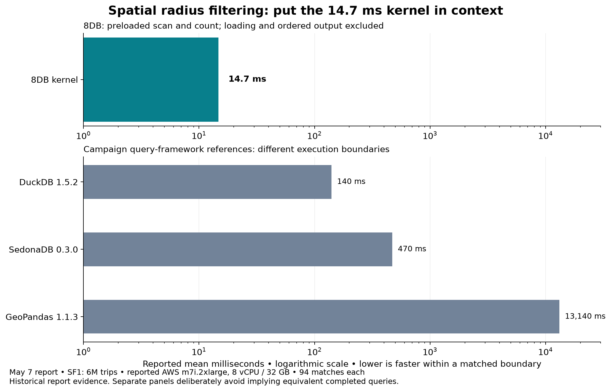
A fleet dashboard repeatedly filtering resident coordinates has a different latency budget from a first query over files. The 14.7 ms result speaks to the former; a cold-file comparison must also charge loading and decoding.
Six million locations: radius-filter references
Milliseconds, lower is better. Fixed zero-to-15,000 scale; very short bars retain their numerical labels.
Preloaded coordinates; filter and count. 94 matches reported.
Query path; Parquet-backed inputs and returned results in reconstructed timer. 94 matches.
Query path; Parquet-backed inputs and result conversion in reconstructed timer. 94 matches.
Query path includes loading, filtering, sorting and projected results. 94 matches.
A different representation changes the performance question
The SF1 report also records a later Hilbert-window candidate path at 0.77 seconds, compared with the original 5.20-second R-tree path. That result is exploratory: neighbor identity and recall were not validated. It shows a promising search strategy to qualify, not an established accuracy-equivalent improvement.
A separate May 8 experiment explored five paths on an M1 Pro with 16 GB RAM and AC power. Its 41 million TLC-derived records used repeated zone-centroid locations. Across three recorded trials per path, the means ranged from 18.40 seconds for R-tree to 2.51 seconds for MERA.
Open the original candidate-path chart.
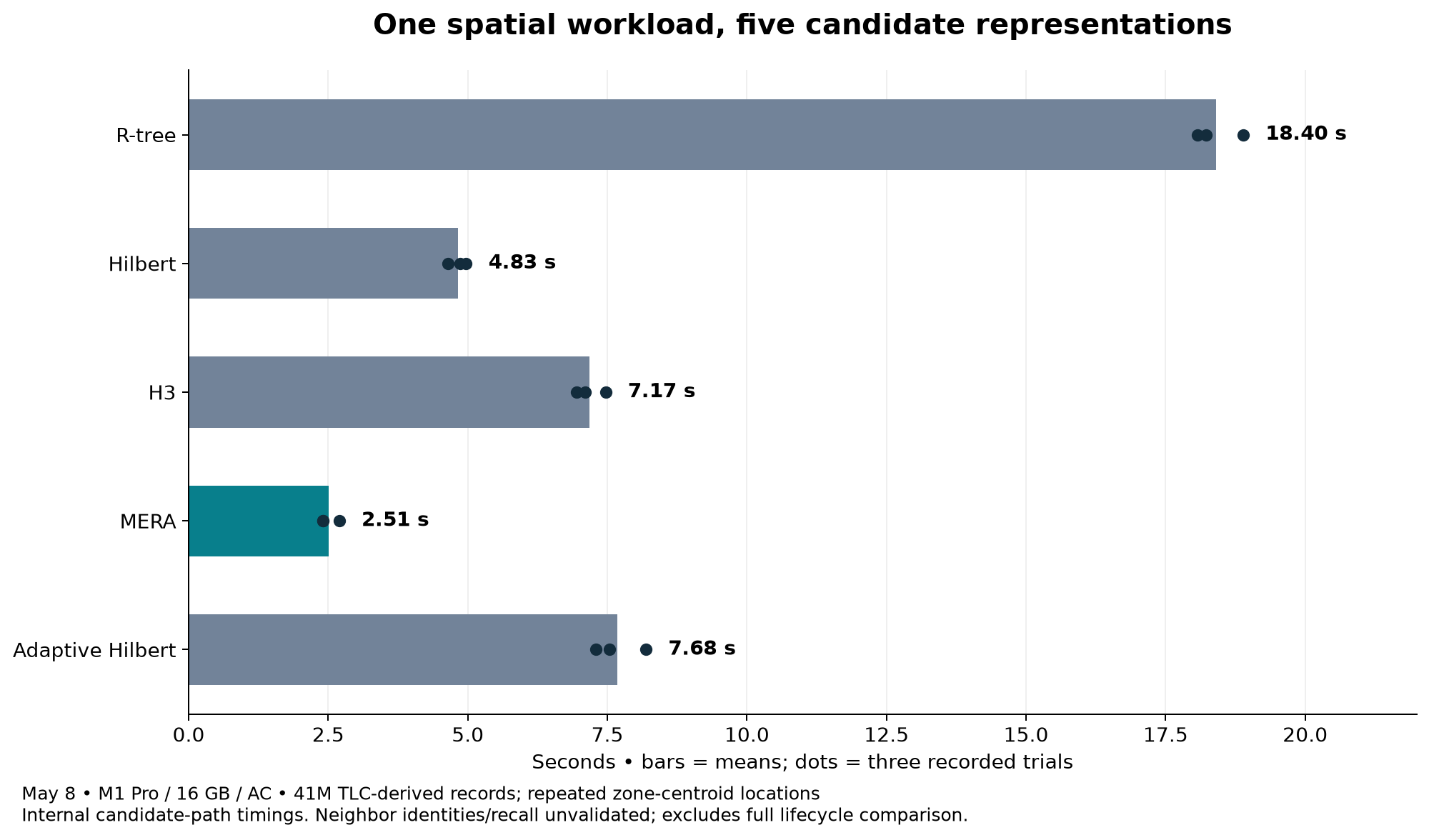
This is a different dataset and hardware configuration from SF1. Neighbor identities and recall remain unvalidated, and full build-and-output costs need separate accounting. The useful insight is that representation can materially change execution time; matching answer quality is the next test. May 8 report.
Five candidate paths, with every recorded trial
Approximately 41M TLC-derived trips with repeated zone-centroid locations. Mean seconds, lower is better.
Three recorded trials: 18.8904 s · 18.0725 s · 18.2304 s
Three recorded trials: 4.9710 s · 4.8607 s · 4.6490 s
Three recorded trials: 7.4682 s · 7.0997 s · 6.9526 s
Three recorded trials: 2.6971 s · 2.4102 s · 2.4086 s
Three recorded trials: 8.1914 s · 7.5396 s · 7.2946 s
Where the specialists fit
The published September 2025 SpatialBench reference supplies broader context on the same named instance class. Its full-query timings include loading Parquet from S3, using different versions from our local campaign.
| Published SF1 result | SedonaDB 0.1.0 | DuckDB 1.4.0 | GeoPandas 1.1.1 |
|---|---|---|---|
| Q1 radius filter | 0.66 s | 0.96 s | 12.78 s |
| Q12 nearest-neighbor join | 14.55 s | Error | Timeout |
The published timeout is 1,200 seconds, distinct from our campaign's 600-second limit. Errors and timeouts describe those tested versions and configurations. The table is a separate reference, not a matched ranking against 8DB's kernels. Published results and methodology.
Capability matters alongside speed. PostGIS offers 3D predicates, n-D bounding-box indexing and advanced geometry through SFCGAL. DuckDB represents Z/M geometry, while SedonaDB has geometry and raster functions. We have no matched PostGIS timing in this recovered campaign. PostGIS indexing, advanced geometry, DuckDB geometry, SedonaDB functions.
Location is one part of the decision
8DB is an omnimodal database. Our spatial source review found n-dimensional metric and in-memory index primitives, point-cloud region and nearest-neighbor queries, multiband raster operations, and persistent GeoQL local charts. Their integration and validation maturity differ; these benchmarks do not measure all those capabilities or establish complete GIS parity.
Consider selecting a service vehicle. Location finds nearby candidates. Telemetry tells you which are available. History informs reliability. Relationships identify the technician with the right certification. Spatial performance becomes more valuable when it helps answer that whole question.
Keeping these operations within one engine could reduce synchronization work, duplicated data and delays between a new observation and a useful answer. Those are deployment-dependent opportunities, not measured savings from this campaign. The relevant comparison is the complete workflow, including the capabilities and integrations needed to deliver it.
Our articles on key-value performance, time-series ingestion and analytical querying explore other native modalities and their own measured conditions.
The spatial results give us something worth building on: a millisecond filtering core, seconds-scale candidate search and several representation choices. Bring us the location query your application needs, its dataset size and its freshness requirement. Include the returned geometry or neighbor identities your application must receive. Let's compare the full path from spatial data to a decision.